Quantum computers and their capabilities is an area of growing global interest and resource allocation. Particularly exciting is the possibility of exponential improvements in classical machine learning algorithms when executed by an equivalent algorithm on a quantum computer. GWDG, along with ZIB and PC2, had the opportunity to provide a window into the world of quantum computing and quantum machine learning at the ISC2023 Conference. We gave demonstrations how quantum computers are programmed today, using an accessible Python framework like Qiskit, developed by IBM Quantum. While GWDG does not currently offer access to real quantum devices, Qiskit includes a powerful simulator, which we packaged into a container you can access from our Jupyter-Hub HPC instance.

You can use this pre-installed environment to start your own quantum computing experiments, for example with our tutorial material.

Tutorial Overview

The range of topics covered start from basic terminology and structures in quantum computing, and end at the rather promising concept of hybrid quantum-classical machine learning algorithms, particularly the Variational Quantum Classifier. Everything presented is oriented towards near-term value regarding quantum computing capabilities.

All resources can be found in the tutorial repository.

Section 1 – Quantum Computing Basics

The concept of quantum computers is only 40 years old, and the first (Nuclear Magnetic Resonance (NMR) based) quantum computer was realized in 1998. Then in 2016, the first system was made available to a broader public. Currently the largest quantum computer holds 433 qubits, with that amount is doubling or tripling every year. That many qubits is much more than necessary in this tutorial, but commercial quantum advantage is speculated only at a hundred thousand qubits, or even millions. Qubits can be made utilizing superconducting circuits, photons, trapped ions, quantum dots, and other methods; each providing their own advantages and disadvantages.

But what is a qubit anyway? In a nutshell, a qubit can be expressed as a 3-dimensional unit vector pointing in an arbitrary direction. If it points „straight up“, it is similar to a classical 0 bit, written $|0⟩$, and „straight down“ would be a classical 1 bit, written ∣1⟩. These are called computational basis states. Pointing anywhere else is a superposition of these states, meaning a linear combination with (complex) coefficients:

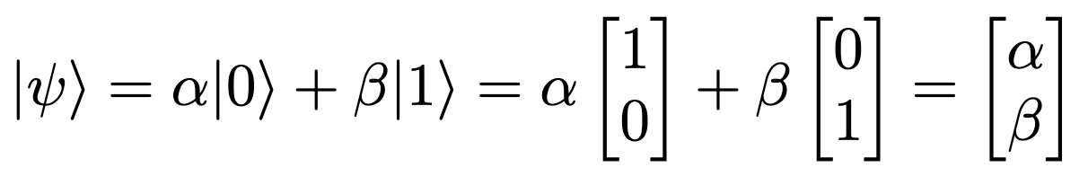
$\alpha ,\beta$ are complex numbers (2 complex numbers can map a 3D-space). We can put multiple qubits together to create higher dimensional information spaces, and we can apply 1-qubit and 2-qubit gates/operations to the qubits to rotate and entangle them. Qubits and gates form quantum programs, called quantum circuits. Quantum entanglement means that qubits in an entangled group cannot be described independently; if you measure any one qubit, the result immediately determines the outcome of measuring another from the group. Measuring a qubit results in its state collapsing to a ∣0⟩ or a ∣1⟩ with a probability depending on its state at the time before the measurement – think Schrödinger’s cat!

There is a set of gates that allows us to reproduce the full range of basic operations that classical computers can do, and so quantum computers can perform all classical algorithms (in theory). However, the beauty of superposition and entanglement allows for novel quantum algorithms that could prove advantageous over classical ones. For example, Shor’s algorithm on a noise-free quantum computer can factorize a large number into two prime numbers faster than any classical algorithm on a classical (super)computer. Other notable algorithms are Grover’s algorithm, Quantum Fourier Transform and Quantum Phase Estimation.

Above, we mentioned „in theory“ and „noise-free“. That is because, given current hardware, noise enters quantum algorithms at a certain rate due to decoherence (noise from the environment intruding on the hardware functionality), gate errors, etc. When too much noise is present, measurements become unreliable. This is why the design of QPUs (Quantum Processor Units), their interaction with classical hardware, and techniques like error correction and error mitigation, are essential for reliable computations.

Section 2 – Quantum Machine Learning

Quantum algorithms typically consist of initializing a certain amount of qubits to a desired state, applying many gates, and measuring to receive a classical output. This is often done many times to get a distribution of results, since the measurements are probabilistic with a probability distribution determined by the algorithm. QML algorithms typically add a classical compute component to this, and we get the following structure:

1. Quantum encoding of data – encode classical data into qubits via a feature map.
2. Quantum algorithm – compute a quantum kernel, QNN (quantum neural network), quantum autoencoder, etc. and measure.
3. Classical post processing – for example, use a quantum kernel in a classical SVC, or use a classical optimizer to find the best parameters for a quantum neural network.

 

We will consider 2 cases: (1) a quantum kernel with a classical ML classifier; (2) a quantum classifier with a classical optimizer.

Case 1: We first require a feature map. Our choice of feature map, e.g. Qiskit has PauliFeatureMap, ZZFeatureMap, Custom; and our configuration of said feature map, e.g. repetitions, determines how the classical data is encoded into quantum states. The amount of qubits and parameters depends on the amount of features in the data. We then compute the fidelity, which is the overlap between two quantum states, between all quantum representations of data points in our training set, resulting in a quantum kernel. This kernel is analogous to classical kernels, and can be evaluated into a classical kernel for use in e.g. SVC or Clustering. We could also use a technique called QKA (quantum kernel alignment) with a TrainableKernel to insert parameterized gates into the feature map that can be optimized for better encoding.

Case 2: Here, we once again require a feature map. We then need what is called an ansatz. An ansatz is similar to a feature map in that it is a parameterized circuit, but instead serves to create a quantum neural network. Qiskit has built in ansatzs, such as RealAmplitudes, EfficientSU2, Custom. The amount of repetitions we choose acts similar to the amount of layers in a classical neural network. The entanglement in feature maps and ansatzs can also be chosen, e.g. full, linear or circular. Measuring the output of the ansatz is what will finally give us our classifier model, but for that we need an optimizer to iteratively calibrate the parameters in the ansatz until we achieve the lowest cost. There are a variety of classical optimizers to choose from, e.g. SPSA and COBYLA, and similarly how we define the cost function is up to our own discretion. Such a classifier is called a Variational Quantum Classifier (VQC) and Qiskit even has a callback graph function built into their interpretation of VQC to see how and if the cost stabilizes after the specified iterations.

Prerequisites and setup

The easiest way to get started is via the GWDG Jupyter-HPC platform. After logging in, at Select a job profile:, choose GWDG HPC with own Container and enter the path /scratch/projects/workshops/quantum_computing/ISC23/qiskit.sif to use our predefined qiskit environment. One core is sufficient to run the notebooks. Now you can spawn your server. From there, just git clone the repository and you are good to go!

Resources

https://gitlab-ce.gwdg.de/lourens.van-niekerk/isc-2023-qml-tutorial

The tutorial is a hybrid of slide presentations and hands-on jupyter notebooks with examples and exercises. The two sections, Quantum Computing Basics and Quantum Machine Learning, each have their own slides and notebooks. There is also a Comprehensive Reading pdf explaining in greater detail the content of both sections.

Author

Christian Boehme, Lourens van Niekerk