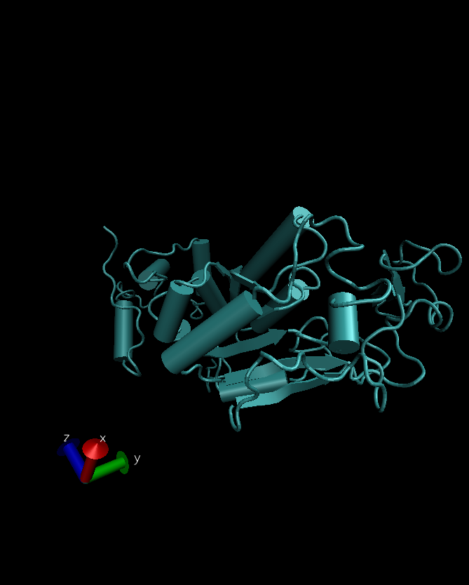
In the realm of computational biology, GROMACS has emerged as a powerful tool for molecular dynamics simulations. Our service provides a detailed guide to setting up and running a GROMACS simulation workflow, complete with visualization using Visual Molecular Dynamics (VMD). For a more detailed workflow please checkout the corresponding README.md file.
Setting Up Your Project
Before you begin, ensure you have a Protein Data Bank (PDB) or AlphaFold output file. This will serve as the starting point for your simulation. Start by creating a new directory for your GROMACS project and add your PDB or AlphaFold output file to the new directory. Clone this git repository and copy the .mdp and .sh files from 20240320_gromacs directory to your GROMACS directory.
Running Your Simulation
To run your simulation, use the following command:
sbatch gromacs.sh 15 13
The first input (15) is for choosing the force field. The second input (13) is for the selection of a continuous group of solvent molecules.
Analyzing Results with Grace
The output of the script will contain several *.xvg files. To visualize the respective graphs, load the necessary modules (gromacs/2023.3-cuda and grace/5.1.24) and run xmgrace with your intended file. You can then save your images in your desired format.
Visualization with VMD
For more experience, visualize your simulation results with VMD. Create and activate a new conda environment, install VMD, and launch it with your .gro file. Inside VMD, set the visualization type and the representation to your desired choice.

GROMACS Simulation: File Summary and Indicators of a Good Simulation
In a GROMACS simulation, various files are generated at different stages, each serving a specific purpose. Here’s a summary:
File Types
– mdp files: These Molecular Dynamics Parameter files provide the settings for each stage of the simulation. We initially provide these files. Examples include minim.mdp for energy minimization, nvt.mdp for temperature equilibration, and npt.mdp for pressure equilibration.
– tpr files: These binary run input files are generated by grompp. They contain the starting structure of your system, the molecular topology, and all the simulation parameters. Examples include em.tpr, nvt.tpr, and npt.tpr.
– trr files: These trajectory files store the coordinates, velocities, and forces for every atom in your system at every time step of the simulation. Examples include em.trr, nvt.trr, and npt.trr.
– cpt files: These checkpoint files allow you to continue a simulation from where it left off. Examples include nvt.cpt and npt.cpt.
– log files: These files contain a detailed record of the simulation, including performance statistics and messages from GROMACS. Examples include em.log, nvt.log, and npt.log.
– gro files: These GROMOS87 format files contain the atomic coordinates of your system. Examples include em.gro, nvt.gro, and npt.gro.
– edr files: These energy files store the energies, temperature, pressure, box size, density, and virials of your system in a binary format. They are generated during your simulation and can be analyzed using the GROMACS energy module. Examples include npt.edr, nvt.edr, and em.edr.
– posre file: This position restraint file is used to restrain the movement of certain atoms in the system during the simulation. This can be useful in equilibration stages where you want parts of your system to settle down without significant conformational changes.
– topol files: These topology files contain the molecular structure of your system, including atom types, bonds, angles, dihedrals, and non-bonded parameters. They are essential for defining the chemical properties of your system.
– xvg files: These output files from GROMACS analysis tools contain data plotted in graphs. They can be visualized using tools like Xmgrace. Examples include density.xvg, gyrate.xvg, potential.xvg, pressure.xvg, rmsd.xvg, and temperature.xvg. The content of each xvg file depends on the specific analysis tool that generated it. For example, an xvg file generated by gmx rms would contain root-mean-square deviation (RMSD) values over time.
Indicators of a Good Simulation
The signs of a good GROMACS simulation can vary depending on the specific system and simulation parameters. However, here are some general indicators:
– Energy Conservation: In a microcanonical (NVE) ensemble, the total energy of the system should be conserved.
– Stable Physical Quantities: Quantities like temperature, pressure, and density should reach equilibrium and fluctuate around mean values in an NVT or NPT ensemble.
– RMSD Plateau: The root-mean-square deviation (RMSD) of the atomic positions from a reference structure should reach a plateau, indicating that the system has equilibrated.
– No Large Forces: There should not be any large forces acting on the atoms, which could indicate bad contacts or high energy conformations.
– Sufficient Sampling: The simulation should be long enough to sufficiently sample the phase space of the system.
For more information, you can refer to this tutorial. If you encounter any issues, please let us know. We’re here to help! Happy simulating!
Author
For any questions, don’t hesitate to contact us via mail: agc@gwdg.de
